Lightweight Time Travel Analysis with Frida: faster Android emulation

We believe that full-system emulation of Windows, Linux, and Android is a powerful way to perform advanced analysis, like Time Travel Analysis. That is why we built it into our esReverse tool. However, in some cases, emulating an entire system can be overkill, creating large traces that slow down investigations.

With this in mind, our team worked on adding time travel debugging support for the Unicorn and Qiling emulators, which can help simulate processors and system behavior accurately. This made it possible to combine emulation and Time Travel Analysis in a single setup.

We have already shown how we found and exploited a vulnerability in a Linux-based target router using Qiling. But what about Android? These methods have limits when dealing with mobile apps, which often need a real device to function properly.

So when Synacktiv's team did an outstanding job open-sourcing Frinet, using Frida as a tracer to generate Tenet-compatible traces, we thought: "That’s awesome! Let's see how leveraging Frida for tracing can apply to our own time travel analysis solution..."

And here we are!

Android Mobile Applications as a Use Case

When analyzing Android applications, we often need to trace specific parts of their execution, such as cryptographic operations, Runtime Application Self-Protection (RASP) behaviors, or unpacking processes.

In some cases, emulation is not an option. Many apps depend on real device features that are unavailable in an emulator. For example, applications using hardware-based security (TrustZone, SIM card, Bluetooth, fingerprint sensors, etc.) may not function properly in a virtual environment.

To solve this, we created an alternative method.

Our solution allows users to generate time travel analysis traces while choosing the tracing method that works best for them.

Meaning you can use a tracer on a real Android device to collect execution data and still produce valid time travel traces for esReverse. This way, you get the best of both worlds: access to real-device behavior while keeping the power of time travel debugging!

One Library to Support All Tracers

So, if you already have a tracing method that works for you, whether through emulation or by instrumenting a real device, you can easily integrate it with our trace generation library. This makes it possible to create time travel analysis-compatible traces for use with esReverse.

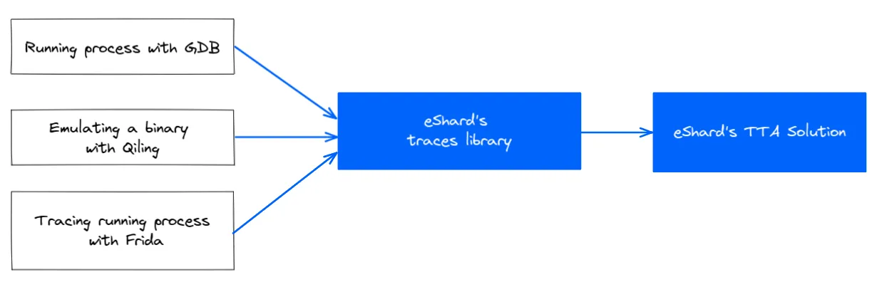
To generate a valid Time Travel Analysis trace, the tracer must provide key details to our library, including:

• Memory mapping: The layout of the target's memory, including linked libraries, their locations, the heap, the stack, and binary sections.
• CPU context: A representation of each CPU register's state at every instruction execution.
• Memory access: Information on whether an instruction reads or writes to memory, and if so, the exact data being written.

To make integration simple, we provide a lightweight API that lets users implement these features with minimal effort.

Now, it is time to see how this works in a real-world scenario. Our use case focuses on tracing an Android mobile app’s native library on a real device.

As we explained earlier, we are leveraging Frida as our tracer, based on the work Synacktiv did with Frinet.

Android Mobile App vs Lightweight Time Travel Analysis

Back to our main goal: tracing an Android mobile app's native library on a real device. To achieve this, we simply integrate our Frida tracer into the application. The Stalker (our tracer) collects all CPU and memory modifications and sends them to our main Python script. This script acts as a bridge between our tracer and the trace library.

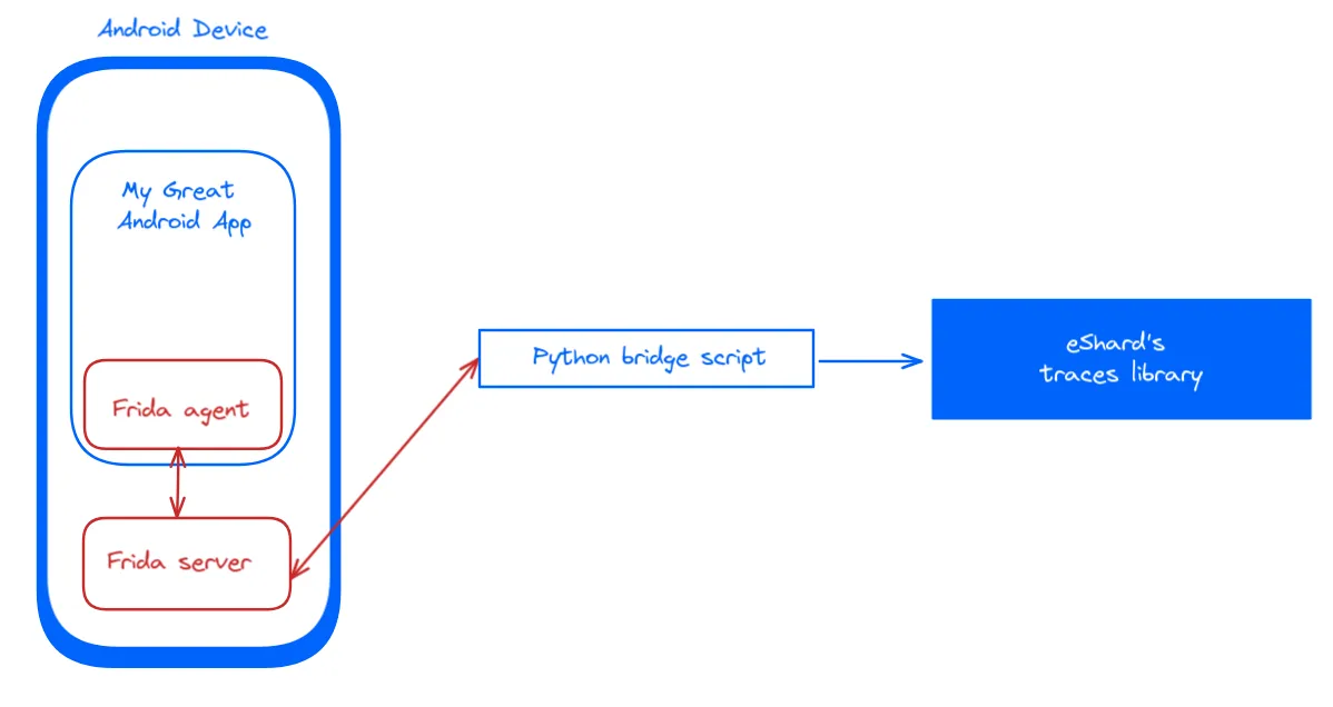
We won't get into details regarding the implementation of the tracer (the red blocks in the graphic), however let's describe how using Frida to determine when to start tracing helps eliminate unnecessary noise from our analysis.

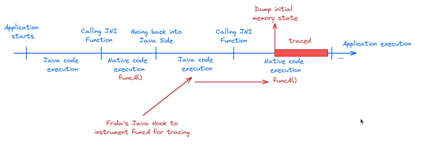
For example, suppose we want to trace the native function funcA() inside a native library. However, funcA() might be called multiple times throughout the application's lifecycle. To target the exact call we're interested in, we can use Frida hooks to trigger tracing at the right moment.

When the targeted call occurs, we first dump the initial memory state we need (heap, stack, binary mapping in memory, etc.). Then, we let the execution proceed under our tracer until we reach the end of our target scope.

To test our solution, we propose tracing the OWASP UnCrackable L2 application. This app presents a text input field where users must enter a hidden flag. If you're already familiar with this challenge, you know that performing time travel analysis isn't strictly necessary to solve it.

However, the goal of this blog post isn't to demonstrate how Time Travel Analysis helps solve a problem, but rather how to accelerate the analysis process.

During the static analysis of the application, we quickly identify a library called libfoo.so, which provides a JNI function responsible for checking the flag. We determine that the function Java_sg_vantagepoint_uncrackable2_CodeCheck_bar is located at offset 0x0dac.

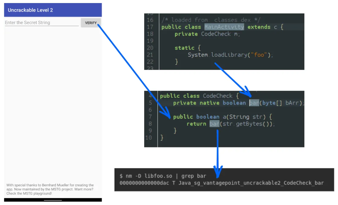
With this information, we can structure our Frida script to look something like this:

// ...
// define the function trace() and the CModule tracer
// ...


Java.perform(() => {
   // Java hook to prepare our "tracing hook".
   let MainActivity = Java.use("sg.vantagepoint.uncrackable2.MainActivity")
   MainActivity["onCreate"].implementation = function (bundle) {
       try {
           let libso = Process.findModuleByName("libfoo.so");
          
           // Hook the function Java_sg_vantagepoint_uncrackable2_CodeCheck_bar and trace its execution
           Interceptor.attach(libso.base.add(0x0DAC), {
               onEnter(){
                   trace(this.threadId)
               },
               onLeave(){
                   const trace_end = new NativeFunction(c_mod.send_end, 'void', []);
                   send("Tracing is finished.");
                   trace_end()
               }
           })
       } catch (e){
           console.log(e.stack)
       }
       this["onCreate"](bundle);
   };
})

On the Python side, we handle the various events received—such as memory access and CPU states—to populate our trace.

At the end of execution, we obtain the following trace files:

• trace.bin and trace.cache – These contain the main data, including CPU contexts, memory region definitions, and more.
• memhist.sqlite – This stores the complete history of all memory read/write operations.

Now, let's take a look at our trace with our time travel debugging tool!

Enjoying our trace with esReverse

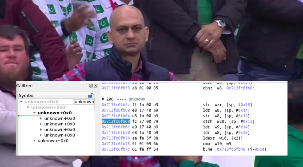
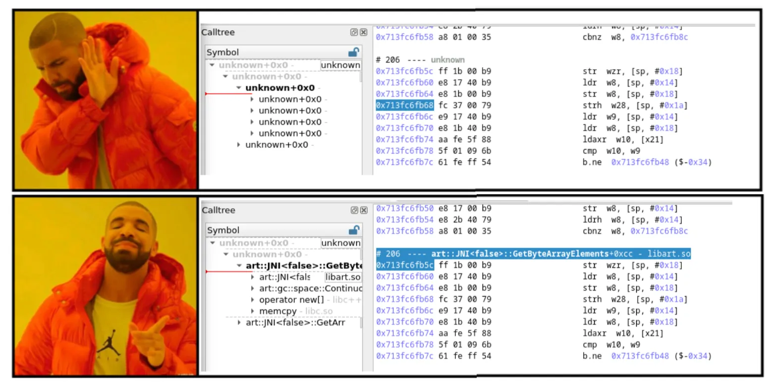
Well... this isn’t quite what we were expecting, right? But wait, don’t run away! We can explain everything!

When performing full-system time travel analysis, esReverse handles 99% of the work for you: gathering system libraries, symbols, and more.

However, with lightweight time travel analysis, we need to manually enrich the trace with additional information. Let’s explore some simple techniques to enhance our trace and achieve the level of quality we deserve.

Enhancing the trace - user modules

The first enhancement provided by the esReverse time travel debugging tool is the user_modules.json file. This file defines the memory mapping of our process, allowing for better trace representation.

Simply put, it provides a structured view of the process's memory layout. It looks like this:

{
   "modules": [
      
       {
           "path": "/path/to/binary/in/traced/system",
           "base_address": "0xBBBBBBBBBB",
           "size": 847872
       },
       ...
   ]
}

This allows the tool to determine which module a given instruction belongs to.

Fortunately, Frida provides a convenient API for this through its module enumeration. By leveraging this feature at the right moment during execution, we can generate a user_modules.json file that accurately represents the process’s memory mapping.

{
   "modules": [
      
       {
           "path": "/apex/com.android.runtime/lib64/bionic/libc.so",
           "base_address": "0x73d3044000",
           "size": 847872
       },
       ...
       {
           "path": "/data/app/~~xFcq-bOB0e3256mTA-DmfA==/owasp.mstg.uncrackable2-WVhKdUcNdYIP0dEkWQP1jg==/oat/arm64/base.odex",
           "base_address": "0x70d1a01000",
           "size": 827392
       },
       {
           "path": "/data/app/~~xFcq-bOB0e3256mTA-DmfA==/owasp.mstg.uncrackable2-WVhKdUcNdYIP0dEkWQP1jg==/lib/arm64/libfoo.so",
           "base_address": "0x70d08c9000",
           "size": 81920
       },
       ...
   ]
}

Let's restart our time travel debugging tool and see how our trace representation has improved.

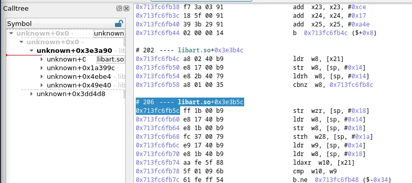
Ah! Much better, isn’t it? We can now see the libraries, but the symbol representation is still far from perfect...

Time for our second trick!

Enhancing the trace - user light fs

The second feature allows us to provide a portion of the file system related to our trace, known as the user light fs.

This file system, combined with the memory mapping of each library and binary, enhances the trace by providing additional context. The esReverse time travel analysis solution parses these binaries to extract public symbols, enriching the trace a posteriori after the tracing step.

For example, we can recreate a portion of the Android filesystem and represent how our application is unpacked within it. As a result, alongside our trace, we obtain a structured filesystem representation like this:

$> tree
.
├── memhist.sqlite
├── trace.bin
├── trace.cache
├── user_modules.json
└── user_light_fs/
   ├── apex
   │   ├── com.android.art
   │   │   └── lib64
   │   │       └── libart.so
   │   └── com.android.runtime
   │       └── lib64
   │           └── bionic
   │               └── libc.so
   ├── data
   │   ├── app
   │   │   └── ~~xFcq-bOB0e3256mTA-DmfA==
   │   │       └── owasp.mstg.uncrackable2-WVhKdUcNdYIP0dEkWQP1jg==
   │   │           ├── base.apk
   │   │           └── lib
   │   │               └── arm64
   │   │                   └── libfoo.so
   └── system
       ├── bin
       │   └── linker64
       └── lib64
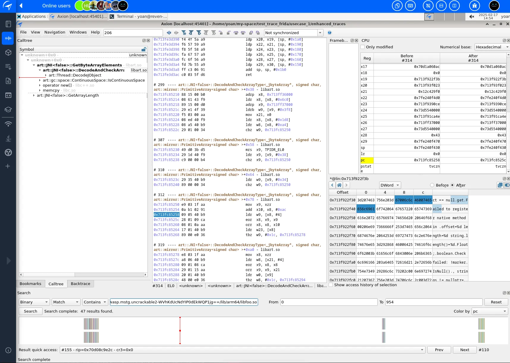
           └── libc++.so

Let's restart esReverse and see how we transformed a raw trace into a much more insightful and structured representation.

And now what? Well, we have a fully exploitable trace for a focused scope of the native execution of the Android application (i.e., the JNI function Java_sg_vantagepoint_uncrackable2_CodeCheck_bar), on a real device, with only 1000 instructions, in less than a minute!

This is helpful to reverse engineer short behaviours like cryptographic operations, Runtime Application Self-Protection (RASP), packers, etc...

If you want to know more on what our time travel debugging tool can help you to achieve, go check out our blog posts like the Tenda crash root cause analysis or our Android full system emulation, for instance.

Full-system vs Lightweight Time Travel Analysis: who wins?

So, in the end, who wins? Well… nobody, and everyone.

It all depends on your needs. If you require an omniscient view of a specific user journey and have the necessary time and storage resources, a full-system time travel analysis is the way to go. You will be able to access any event or instruction that occurred during your recording, on the entire system, including kernel, user-land, and more, directly at hand.

On the other hand, if you need a quick and efficient tool to accelerate your reverse engineering process due to time or resource constraints, lightweight time travel analysis is a strong alternative. It is limited to a small scope of the process you target, it won't trace anything outside your process, but it can provide light results faster.

For further comparison between both solutions, stay tuned, for the next blog post!